How to train MLPs in Scikit Learn and infer in Java
Quite recently, I needed an image classifier for one of my projects. The requirement was for the classification system to filter out a particular class of undesired images from a high speed stream of images. Luckily, the images for the task were simple 16x16 grayscale images, which I figured could be easily processed by a traditional feed forward network. In fact, I was able to verify this in a few hours of tinkering with Scikit Learn, and it appeared my task was actually solved. But there was a problem: the source code for my project was in Java, and my Scikit Learn solution was in Python.

Meet Scikit Learn
I strongly believe Scikit Learn is most data scientists' favourite machine learning toolkit. Although I do not have any evidence to back this claim, anecdotes from several data scientists, and my own personal experiences inform it. And I don't think I'm wrong on this one.
Scikit Learn emphasizes simplicity through a consistent API, and it ships with a vast collection of algorithms that cover almost the entire gamut of machine learning techniques. This batteries included nature makes Scikit Learn my initial go-to whenever I have to evaluate a learning task or analyze data. When using Scikit Learn, you do not need a ton of boiler-plate code, you can easily interchange learning algorithms, and it's so fast that you can quickly iterate through your ideas when working with it.
A Conundrum: How to Scikit in Java
So, back to my problem. With my classification task solved in Scikit Learn, I needed a way to run the Python based solution in my Java code, and I needed to do it without disrupting much. My first thought was to run Scikit through Jython, which is a python runtime for Java. This had been my original plan all along, but it was painfully proven impossible because of Scikit Learn's dependency on Numpy (a powerful numeric library for python) which is written in C and cannot be executed in the JVM. Another option was to port the entire project to Python. This was a big no no, given the maturity of the project and the small (but important) role the classifier was meant to play. I also thought of using other Java ML libraries like Weka, but I was so spoiled by the simplicity of Scikit Learn, I wasn't willing to put in the extra effort to redo something that had already been done. Heck, I even considered Tensorflow for Java, but that's an entirely different story.
Stuck with very few options, and looking for an elegant way out, it dawned on me: Maybe I could train the network in Scikit Learn, export the weights and write a small inference engine in Java to use in my project. Although this sounds complicated, it's actually quite simple, and so it's exactly what I did! In this post I'll be describing the entire process.
For the examples in this post, we'll use the MNIST dataset (a simple dataset that's incredibly close to what I was working with) and we will write an inference engine in Java using OpenCV as a numeric library. Maybe, someday, I'll make an updated post that uses Apache Commons Math as the numerical library.
Some Background
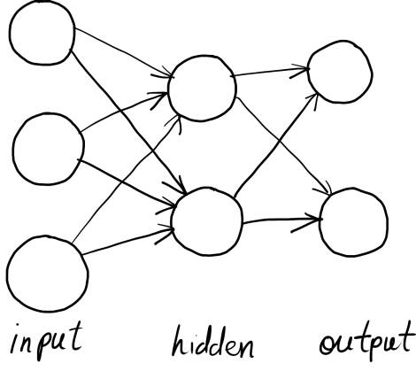
Before we get coding, let's cover some background material for this work. The neural network model used in Scikit Learn's MLP classifier is your standard off the conveyor belt feed-forward neural network. It has an input layer of nodes, an output layer, and a series of inner, hidden layers. Nodes on each layer are fully connected to those on the previous layer, and each node computes a weighted sum of each of its inputs, which is offset by a bias value before it's passed through an activation function.
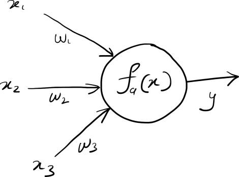
Mathematically, the computation at each node can be represented as:
$$y = f_a(w_1 x_1 + w_2x_2 + ... + w_nx_n + b)$$
Here $y_i$ represents the output of the node, $x_1$ through $x_n$ represent the inputs to the layer, $w_1$ through $w_n$ represent the weights for each input, and $b$ represents a bias (or an intercept) of the node. $f_a(x)$ is a special function, known as the activation function, which determines the final output of the node.
One interesting advantage of representing the network this way is that we can perform all the computations of any layer as a single matrix multiplication. As such, if we consider all the weights of a given layer as a matrix $W$, and all the inputs as a vector $X$, we can obtain all the activations for any layer as: $$Y = f_a(W \cdot X + B)$$
Assuming our input vector, $X$, is of size $m$ and the layer for which we are computing has $n$ nodes, then our weights matrix $W$ will have $m$ rows and $n$ columns, and our bias and output vectors will also be of length $n$.
Having the ability to make the computations this way is really cool because if there's anything modern computers are good at, it's multiplying matrices. This matrix approach also simplifies our inference work (we have to write less code) while allowing us to take advantage of some of these modern computation capabilities. When writing our inference code, we will only need compute the matrix multiplication between our input, $x$, and the weights, $W$, from Scikit Learn, and when we add the biases, $b$, and pass the output through the activation function, $f_a(x)$, and we'll obtain our prediction $y$.
One final piece we need to cover before implementing our inference function, however, will be the choice of activation functions. In Scikit Learn, the activation function depends on the particular layer of the neural network. By default the input and hidden layers have the Rectified Linear Unit, which is computed as:
$$f_{ReLU}(x)=max(x, 0)$$
It's essentially a ramp function that cuts out all negative values and preserves positive ones. And the output layer, on the other hand has a the Sigmoid function:
$$f_{Sigmoid}(x)=\frac{1}{(1 + e^{-x})}$$
The sigmoid is a special function with statistical properties that allow it to significantly suppresses potential errors while significantly boosting predictions. These activation functions are the defaults configured in Scikit Learn, and we can always change them if we want to. Just remember that if we should use any other configuration, we need to implement the same functions in your Java inference code. But these defaults are actually quite reasonable, and they should work well for most learning tasks that'll be thrown at it.
Obtaining the Weights: Training in Scikit
Training a classifier in Scikit is extremely simple. First, we get the data, second we call the fit(x, y) method of our desired classifier, and finally we tune and iterate. For this demonstration, we'll be using a copy of the MNIST dataset packaged in CSV form. This form of the MNIST has each pixels value as a column in a wide spreadsheet. You can find a copy here.
Oncw we have our data, we'll code to reading it into the Numpy arrays Scikit Learn requires. For the inputs ($X$) we'll read the values from the spreadsheet and divide each by 255 to normalize. For the outputs ($Y$) on the other hand, because the spreadsheet provides a single number, we need to encode the output as a one-hot vector covering the 10 possible outputs. Luckily, scikit ships with a one hot encoder we can use for this.
Below is a a simple implementation of a python function to read this data.
import csv
import numpy as np
import sklearn.preprocessing import OneHotEncoder

def read_data(path:str) -> tuple:
    x = []
    y = []

    with open(path, "r") as f:
        reader = csv.reader(f)
        next(reader)
        for row in reader:
            y.append([row[0]])
            x.append(np.array(row[1:], dtype=np.float64) / 255)

    return np.array(x, dtype=np.float64), one_hot_encoder.fit(y).transform(y)
Once our function is in place, we can now import our MNIST data as follows.
train_x, train_y = read_data("mnist_train.csv")
test_x, test_y = read_data("mnist_test.csv")
Then, we can tap into the simplicity of scikit learn to train our neural network classifier. Since we are using MNIST, which is made up of 28x28 images, our input layer already has 784 nodes. We can arbitrarily choose to have two hidden layers of sizes 512 and 128, and our one-hot encoded outputs provide a final set of 10 nodes for the output layer. This architecture can be configured simply in Scikit Learn as shown below:
clf = MLPClassifier(hidden_layer_sizes=(512, 128))Note that we do not specify the sizes of the inputs and outputs, because those will be inferred by Scikit Learn from the dataset. This classifier can then be trained simply by executing the line:
clf.fit(train_x, train_y)We can now save the weights and biases into JSON files that can be moved into Java for inference. The clf object holds the weights and biases in its clf.coefs_ and clf.intercepts_ properties respectively. The following code does just that.
with open(f"weights.json", "w") as weights_file:
        json.dump([x.tolist() for x in clf.coefs_], weights_file)
with open(f"biases.json", "w") as weights_file:
        json.dump([x.tolist() for x in clf.intercepts_], weights_file)
And that's it! We have all we need from Scikit. Next, we'll look at inference in Java.
Inferring from the Weights in Java with OpenCV
Our first step in inference will be to load the weights from Scikit into Java as OpenCV Matrix objects. Because we saved our weights to JSON files, we can rely on Google's Gson library (or whatever your favourite JSON library is) to read in these values. As already discussed, each layer has a weights matrix, and a bias matrix. We do not explicitly need to know the number of nodes each layer has, because its inherently represented in the size of the matrix. Also, we must remember that while the weights are two-dimensional, the biases are stored in a single dimension.
Loading the Weights and Biases
We can first load the biases as follows:
Gson gson = new Gson();
List<Mat> biases = new ArrayList<Mat>();

try (FileReader reader = new FileReader("biases.json")) {
    for(double[] bias: gson.fromJson(reader, double[][].class)) {
        Mat mat = new Mat(bias.length, 1, CvType.CV_64F);
        mat.put(0, 0, bias);
        biases.add(mat);
    }
}
The biases will be read into an array list of 64 bit floating point OpenCV Mat objects.
Similarly, we can load the weights as follows:
Gson gson = new Gson();
List<Mat> weights = new ArrayList<Mat>();

try (FileReader reader = new FileReader("weights.json")) {
    for(double[][] weights: gson.fromJson(reader, double[][][].class)) {
        Mat mat = new Mat(weight.length, weight[0].length, CvType.CV_64F);
        double[] flatWeight = Arrays.stream(weight).flatMapToDouble(Arrays::stream).toArray();
        mat.put(0, 0, bias);
        weights.add(mat.t());
    }
}
The difference between the two loaders is in the dimensions. With biases being single dimensioned, they are relatively easy to read into OpenCV mats without much modification. Weights, however, need to be mapped out into a flat array before being loaded into the Mat object. Even after that, the matrix must also be transposed to get it in the right orientation for matrix multplication.
Making Predictions
Now that the weights and biases are loaded, we can make predictions by iterating through the layers. At each stage of this iteration, we will compute the multiplacation between the input and the weights with the Core.gemm function. Core.gemm performs matrix multipications between arrays and adds on the biases through the OpenCV library. Before the output layer is reached, a Relu activation is applied to all inner layers and their output becomes the input for the next layer. On the final output layer, a sigmoid activation is used instead, and the prediction comes in the form of a one-hot vector.
public Mat predict(Mat x) {
    int i = 0;
    Mat activations = new Mat();
    for (i = 0; i < numberOfLayers; i++) {
        Core.gemm(weights.get(i), x, 1, biases.get(i), 1, x);
        // Compute relu activation for hidden layers only.
        if (i < numberOfHiddenLayers) {
            Core.max(x, Scalar.all(0), x);
        }
    }

    // Sigmoid activation
    Mat output = new Mat();
    Core.exp(x, x);
    Core.reduce(x, output, 0, Core.REDUCE_SUM);
    Core.divide(x, Scalar.all(output.get(0, 0)[0]), output);

    return output;
}
Before we make predictions, though, we need to load our data. Just as we did in python, we can easily put together a function to read in the CSV files from our MNIST dataset. This time, however, we'll be reading into OpenCV Mat objects. The following method takes a path to the MNIST file, reads in the data, and evaluates the classifier on each row.
public double evaluate(String path) throws IOException {
    List<String> rows = Files.readAllLines(Paths.get(path));
    double score = 0;

    for(int i = 1; i < rows.size(); i++) {

        String rowString = rows.get(i);
        int value = Integer.parseInt(rowString.substring(0, 1));
        double[] numbers = Arrays
            .stream(rowString.substring(2).split(","))
            .mapToDouble(Double::parseDouble)
            .toArray();
        Mat row = new Mat(numbers.length, 1, CvType.CV_64F);

        row.put(0, 0, numbers);
        Core.divide(row, Scalar.all(255.0), row);

        System.out.println(predict(row).dump());
    }

    return score;
}
When evaluated, the inference performs at the same rate as the original implementation in python. It's really simple, but whenever you find yourself in a bind, you can always use this approach. Performance was phenomenal for me, and I even boosted it further with a lookup table implementation of the sigmoid function.
Putting it all together
The full python and Java scripts can be found in this gist. Remeber that you must have Scikit Learn installed as a dependency in your python environment, and for the Java environment you need OpenCV. You can find Scikit Learn through pip and OpenCV can be found in Maven. Happy Programming.